Version: 1.2
Date: December 2025
Reference Standard: DNV-RP-F107: Risk assessment of pipeline protection
This document provides a comprehensive technical description of the methodology used in the DORAS (Dropped Object Risk Analysis System) application for creating studies and performing risk assessment calculations. The methodology is based on DNV-RP-F107 standards with enhanced computational approaches for improved accuracy and flexibility.
Table of Contents
- 1. Study Creation and Data Entry Workflow
- 2. Calculation Methodology
- 3. Calculation Engine Architecture
- 4. Results Aggregation and Reporting
- 5. Validation
- Frequently asked questions
- Next steps
- 6. References
1. Study Creation and Data Entry Workflow
1.1 Data Entry Order
The following order is recommended for setting up a complete study for analysis. While the system allows some flexibility in data entry order, this sequence ensures all dependencies are properly established as the study is defined:
The study is the first data definition which must be completed when creating a new study. All subsequent data elements will be associated with this study which you define.
While there are numerous parameters which can be defined for each study and which will control the way that the analysis is conducted and reported, the following are the key parameters that must be defined for the study and which have a material impact on the analysis calculations:
- Study name
- Minimum water depth (meters)
- Maximum water depth (meters)
A study Must have at least one Facility definition, and you may have as many facilities as you want. Facilities are used to add the graphical underlay image to visualize the facilites, targets and the general location where the study is being conducted. An image file must be uploaded for each of the facilities that you define.
The following are the key parameters that must be defined for the facility:
- Facility name
- Facility image width (m)
- Facility image height (m)
- Facility longitude (degrees)
- Facility latitude (degrees)
A study Must have at least one fluid definition, and you may have as many fluids as you need. Fluids will be associated with fluid containing targets and will be used with the release frequency calculations for each fluid.
A study Must have at least one target group definition, and you may have as many target groups as you need. Target groups will be used to organize and aggregate targets and will be used with hit release frequency calculations for each target group.
A study must have at least one target definition, and you may have as many targets as you need. Targets will be used to define the infrastructure targets at risk of being hit by dropped objects and will be used with the hit frequency, damage frequency, and release frequency calculations for each target.
The following are the key parameters that must be defined for the target:
- Target name
- Geographic coordinates
- Target type (steel pipeline, flexible pipeline, umbilical, equipment)
- Target class (Linear, Polygon)
- Physical properties:
- Diameter (millimeters)
- Wall thickness (millimeters)
- Yield strength (N/mm²)
- Protection thickness (millimeters)
- Protection energy absorption (kJ)
- Contained fluid (for release frequency calculations)
A study must have at least one crane definition, and you may have as many cranes as you need. Cranes will be used to define the locations and drop zone areas.
The following are the key parameters that must be defined for the crane:
- Crane name
- Crane type (Crane, Derrick))
- Geographic location (latitude, longitude)
- Drop zone type:
- Single point: Fixed drop location coordinates
- Fixed pattern: Multiple predefined drop points coordinates
- Area: Drop zone defined by polygon boundary coordinates
- Random (closest): Random selection from nearest points coordinates
- Random (any): Random selection from all points coordinates
- Distribution type (Normal, Uniform) - optional
A study must have at least one object definition, and you may have as many objects as you need. Objects will be used to define the dropped objects and will be used in the calculation of drop frequency, excursion distance, and impact energy for each object.
The following are the key parameters that must be defined for the object:
- Object name
- Object class (DNV Class 1-7)
- Object mass in air (kilograms)
- Object length (meters)
- Object width (meters)
- Object height (meters)
- Object volume (cubic meters)
- Object drag coefficient (Cd)
- Object added mass coefficient (Ca)
Each crane must have at least one lift manifest definition, and you may have as many lift manifests as you need for each crane. Lift manifests are used to assign objects to cranes which will be used to determine the location and probability of dropped objects in the study.
The following are the key parameters that must be defined for the lift manifest:
- Associated crane
- Associated object
- Lifts per annum
- Bundle size (number of objects in the lift)
- Drop probability per lift
1.3 Calculation Execution
Once all required data is entered, the calculation process executes in the following sequence:
- Drop Calculations: Calculate lateral deviations, terminal velocities, and kinetic energies for all lift manifests
- Landing Probability Calculations: Calculate probability distributions across distances from the drop point
- Matrix Calculations: Perform high-resolution grid-based probability and frequency calculations
- Damage and Release Calculations: Calculate damage categories (D1,D2,D3) and release frequencies (R0,R1,R2)
2. Calculation Methodology
2.1 Dropped Object Frequency
The annual frequency of each dropped objects is calculated for each lift manifest as follows:
- Ndrops = Annual frequency of drops (drops/year)
- Tperiod = Study period in days
- Nlifts = Number of lifts per annum for this operation
- Pdrop = Probability of drop per lift (dimensionless)
- Nbundle = Number of objects per lift (bundle size)
2.2 Dropped Object Excursion Distance (Lateral Deviation)
The lateral deviation (excursion distance) represents the horizontal distance a dropped object travels from the drop point during its descent through water. This is calculated based on water depth and object cone angle as follows:
- σ1 = One standard deviation lateral deviation (meters)
- h = Water depth (meters)
- θ = Impact angle (degrees), determined by DNV object class
The 2σ and 3σ deviations are calculated as multiples of the 1σ value:
- σ2 = 2 × σ1 (2 standard deviations)
- σ3 = 3 × σ1 (3 standard deviations)
For flat or long objects at water depths greater than 180 meters, the excursion distance is capped at 180 meters for lateral deviation calculations to account for reduced trajectory variability in large depths.
2.2.1 Simple Current Effects (Optional)
When the Simple Current Effects option is enabled and a water current velocity is specified, the application enhances the lateral deviation calculations by accounting for horizontal drift caused by water current during the object's descent. This provides a more realistic assessment of landing dispersion in environments with significant water currents. The calculation conservatively assumes that the current will be flowing in the direction of the object excursion.
Current-Induced Dispersion Calculation
The current-induced horizontal drift distance is calculated based on the fall time and current velocity:
- tfall = Fall time through water column (seconds)
- h = Water depth (meters)
- vT,avg = Average terminal velocity (m/s), calculated as the mean of minimum and maximum terminal velocities based on minimum and maximum projected object surface areas
- dcurrent = Horizontal drift distance due to current (meters)
- vcurrent = Water current velocity (m/s)
- tfall = Fall time from Equation 2a (seconds)
Statistical Combination via Quadrature Addition
The current-induced dispersion is treated as an independent source of variability and is combined with the base lateral deviation using quadrature addition (also known as root-sum-square or RSS). This statistical method properly combines independent standard deviations:
- σ1,combined = Combined one standard deviation lateral deviation (meters)
- σ1,base = Base DNV lateral deviation from Equation 2 (meters)
- dcurrent = Current-induced drift distance from Equation 2b (meters)
Multi-Sigma Recalculation
After calculating the combined 1σ lateral deviation, the 2σ and 3σ deviations are recalculated as multiples of the adjusted value:
σ3,combined = 3 × σ1,combined
- σ2,combined = Two standard deviations lateral deviation with current (meters)
- σ3,combined = Three standard deviations lateral deviation with current (meters)
Configuration and Activation
Simple Current Effects are activated when:
- The study's Current Option is set to
"Simple current effects" - The study's Water Current Velocity is greater than 0 m/s
- Terminal velocity calculations are available (valid object mass, volume, drag coefficient, and projected object surface area)
Enabling Simple Current Effects results in:
- Increased lateral deviations: All σ values (1σ, 2σ, 3σ) increase to account for horizontal drift
- Expanded probability footprints: Landing probability distributions spread over larger areas
- Modified hit frequencies: Changes in spatial distribution may increase or decrease target hit frequencies depending on target locations relative to drop points and current direction
2.3 Dropped Object Landing Probability
The probability of an object landing at a specific distance from the drop point is modeled using a normal (Gaussian) distribution. The cumulative distribution function (CDF) is used to calculate probabilities within concentric rings:
- F(R) = Cumulative probability at distance R
- R = Distance from drop point (meters)
- μ = Mean of distribution (typically 0 for centered drop)
- σ = Standard deviation (lateral deviation σ1)
- erf = Error function
For a ring between distances Rmin and Rmax, the probability is:
The probability density (probability per square meter) within the ring is:
- Aring = Ring area = π × (Rmax² - Rmin²)
For a cell of area Acell within the ring, the landing probability is:
2.4 Target Hit Probability
The conditional probability of hitting a target, given that an object lands in a specific cell, is calculated based on the target area exposed within that cell. The target area is adjusted to account for object breadth:
- Ltarget = Target length within cell (meters)
- Dtarget = Target diameter (meters)
- Bobject = Object breadth (maximum of length, width, or height) (meters)
For polygon targets (equipment), the adjusted area includes the perimeter contribution:
- Atarget = Original polygon area (square meters)
- Ppartial = Partial perimeter within cell (meters)
The conditional hit probability for a cell is:
- pcell = Landing probability density in cell (per m²)
- Σ(Atarget,adj) = Sum of all adjusted target areas in cell
2.5 Target Hit Frequency
The annual frequency of target hits is calculated by multiplying the conditional hit probability by the drop frequency:
- fhit = Annual hit frequency (hits/year)
- Phit|landing = Conditional hit probability (from Equation 9)
- Ndrops = Drops per annum (from Equation 1)
Hit frequencies are aggregated across all cells, objects, lifts, and cranes to provide total hit frequencies for each target, object, lift, and crane.
2.6 Target Hit Energy Frequency
The hit frequency is distributed across energy levels using one of two available methods, selected at the study level. Both methods distribute hits across the same six energy level bands defined by DNV-RP-F107:
| Energy Level | Energy Range (kJ) | Description |
|---|---|---|
| 1 | 0 - 50 | Low energy impacts |
| 2 | 50 - 100 | Moderate energy impacts |
| 3 | 100 - 200 | Medium-high energy impacts |
| 4 | 200 - 400 | High energy impacts |
| 5 | 400 - 800 | Very high energy impacts |
| 6 | 800+ | Extreme energy impacts |
2.6.1 DNV Probability Distribution Method
The DNV Probability Distribution Method (default) distributes hit frequencies across energy levels based on fixed probability distributions from DNV Table 5-4. Each DNV object class (1-7) has a predefined probability distribution that is independent of the object's actual calculated kinetic energy. This method provides a standardized approach based on object categorization.
- fhit,level = Hit frequency at energy level (hits/year)
- fhit,object-target = Total hit frequency for object-target pair (hits/year)
- Pclass,level = Fixed probability of energy level for object class (from DNV Table 5-4)
- Uses fixed probability distributions per DNV object class (1-7)
- Energy distribution is based on object category, not actual calculated kinetic energy
- Provides consistent, standardized results across similar object classes
- Recommended when object-specific energy calculations are not available or when following standard DNV methodology
2.6.2 Calculated Effective Energy Method
The Calculated Effective Energy Method distributes hit frequencies using a log-normal probability distribution based on the object's actual calculated effective impact energy values (minimum and maximum). This method uses the object's specific physical properties (mass, drag coefficient, terminal velocity, added mass) to determine energy distribution, providing more accurate and object-specific results.
The log-normal distribution is used because energy values are always positive and typically exhibit right-skewed distributions. The distribution parameters are derived from the calculated energy bounds:
- Emean = Geometric mean effective impact energy (kJ)
- Emin = Minimum effective impact energy (kJ) from object calculations
- Emax = Maximum effective impact energy (kJ) from object calculations
μ = ln(Emean) - σ² / 2
- σ = Log-normal distribution sigma parameter (treats min/max as ±3σ, 99.7% confidence interval)
- μ = Log-normal distribution mu parameter
- Plevel = Probability for energy level (dimensionless)
- CDF = Cumulative distribution function of log-normal distribution
- Emin,level = Minimum energy for level (kJ)
- Emax,level = Maximum energy for level (kJ)
- fhit,level = Hit frequency at energy level (hits/year)
- fhit,object-target = Total hit frequency for object-target pair (hits/year)
- Plevel = Probability of energy level from log-normal distribution
- Uses actual calculated effective impact energy values (min/max) based on object physics
- Applies log-normal probability distribution across the 6 DNV energy bands
- Provides object-specific energy distributions that reflect actual terminal velocity and impact energy calculations
- Automatically screens floating objects (zero energy) when this method is selected
- Recommended when accurate object-specific energy calculations are available and more precise risk assessment is required
2.6.3 Cumulative Hit Energy Frequency
For both methods, cumulative hit energy frequencies are calculated as the sum of frequencies at or above each energy threshold:
- fhit,cumulative,level = Cumulative hit frequency at or above energy level (hits/year)
- fhit,i = Hit frequency at energy level i (hits/year)
2.7 Target Damage Frequency
Damage frequencies are calculated using proportional energy distribution methodology. Hits are distributed across damage ranges based on energy level overlap with target-specific energy thresholds.
2.7.1 Energy Threshold Calculation (Steel Pipelines)
For steel pipeline targets, energy thresholds are calculated using DNV Equation (3) based on target-specific properties:
- E = Absorbed energy (kJ)
- mp = Plastic moment capacity = ¼ × σy × t² (N·mm)
- D = Steel outer diameter (mm)
- t = Wall thickness (mm)
- σy = Yield stress (MPa)
- δ/D = Dent depth / diameter ratio (0.05 for 5%, 0.10 for 10%, etc.)
Energy thresholds are calculated for 5%, 10%, 15%, and 20% dent categories. If protection capacity is specified, it is added to the steel-only thresholds to obtain total energy thresholds.
2.7.2 Proportional Energy Distribution
Hits from each energy level are distributed proportionally across all overlapping damage ranges based on the proportion of the energy range that falls within each threshold range:
- fhit,range = Hit frequency in damage range (hits/year)
- Overlaplevel,range = Overlapping portion of energy level with damage range (kJ)
- Rangelevel = Total width of energy level range (kJ)
2.7.3 Damage Category Frequencies
Damage frequencies for each category (D1, D2, D3) are calculated by multiplying hit frequencies in each range by the conditional probabilities from DNV tables:
- fdamage,Dx = Damage frequency for category Dx (D1, D2, or D3) (events/year)
- PDx|range = Conditional probability of damage category Dx given hit in range (from DNV Tables 4-1, 4-2, or 4-3)
Damage categories are defined as:
- D1 (Minor Damage): Superficial damage, no structural integrity impact
- D2 (Moderate Damage): Moderate structural damage requiring repair
- D3 (Major Damage): Severe structural damage, potential for immediate failure
2.8 Target Release Frequency
Release frequencies are calculated only for targets containing hydrocarbon fluids (not applicable to umbilicals). The calculation follows the same proportional distribution methodology as damage frequencies:
- frelease,Rx = Release frequency for category Rx (R0, R1, or R2) (events/year)
- PRx|range = Conditional probability of release category Rx given hit in range (from DNV Tables 4-1 or 4-2)
Release categories are defined as:
- R0 (No Release): No fluid release occurs
- R1 (Minor Release): Small leak, limited environmental impact
- R2 (Major Release): Significant release, potential for major environmental impact
Umbilical targets do not contain hydrocarbon fluids, therefore all release frequencies (R0, R1, R2) are set to zero for umbilical targets.
3. Calculation Engine Architecture
3.1 Matrix-Based Grid System
The DORAS application uses a high-resolution cellular grid system for probability and frequency calculations. This approach provides significant advantages over traditional concentric ring methods:
- Higher Resolution: Cell sizes can be configured down to 1m × 1m
- Spatial Accuracy: Precise target intersection calculations within each cell
- Cumulative Analysis: Simultaneous processing and accumulation of contributions from multiple drop sources
- Flexible Geometry: Support for complex and irregular target shapes (linear, polygon)
3.2 Calculation Optimization
The calculation engine includes the following performance optimizations:
- Bounding Box Pre-filtering: Spatial bounding boxes eliminate 70-90% of unnecessary target intersection calculations
- Statistical Sampling: Automatic sampling when drop frequencies exceed 10,000 per lift to maintain calculation speed
- Stochastic Loop Averaging: Multiple iterations with averaging for improved accuracy in high-frequency scenarios
3.3 Kinetic Energy Calculations
Kinetic energy calculations are performed as follows:
- vT = Terminal velocity (m/s)
- g = Gravitational acceleration = 9.81 m/s²
- m = Object mass (kg)
- V = Object volume (m³)
- ρw = Seawater density = 1025 kg/m³
- CD = Drag coefficient
- A = Projected area (m²)
- ET = Kinetic energy at terminal velocity (kJ)
- EE = Effective impact energy (kJ)
- ma = Added mass = ρw × Ca × V (kg)
- Ca = Added mass coefficient
Both minimum and maximum kinetic energies are calculated based on minimum and maximum projected object surface areas to establish energy bounds for risk assessment.
4. Results Aggregation and Reporting
4.1 Aggregation Levels
Results are calculated and aggregated at multiple levels:
- Cell Level: Individual grid cell probabilities and frequencies
- Target Level: Per-target hit, damage, and release frequencies
- Target Group Level: Aggregated frequencies for target groups
- Object Level: Per-object hit frequencies and energy distributions
- Lift Level: Per-lift hit frequencies
- Crane Level: Per-crane hit frequencies
- Study Level: Total study-wide frequencies
4.2 Visualization Outputs
The application generates multiple visualization layers in downloadable GeoJSON format:
- Landing probability distributions
- Landing frequency distributions
- Target hit frequency heat maps
- Damage severity visualizations (color-coded by D1/D2/D3)
- Drop cone visualizations (1σ, 2σ, 3σ)
5. Validation
5.1 Validation Methodology
The DORAS application's calculation methods and implementation have been validated through systematic comparison against the worked example provided in DNV-RP-F107 Appendix A. This validation process ensures that all calculation methodologies, equations, and computational approaches implemented in the application produce results that are consistent with the standard's published example calculations.
The validation process involves:
- Replication of DNV Worked Example: The exact scenario from DNV-RP-F107 Appendix A is created in the application
- Calculation Execution: All calculation steps are performed using the application's calculation engine
- Result Comparison: Calculated results are compared against the DNV worked example results at each calculation stage
- Verification of Methodology: Each calculation step is verified to ensure proper implementation of the DNV equations and methodologies
The DNV-RP-F107 Appendix A worked example provides a complete end-to-end risk assessment scenario including:
- Object definitions with physical properties
- Target definitions (steel pipeline) with geometric and material properties
- Drop frequency calculations
- Lateral deviation (excursion distance) calculations
- Landing probability distributions
- Hit frequency calculations
- Energy level distributions
- Damage frequency calculations using proportional energy distribution
- Release frequency calculations
5.2 Validation Results
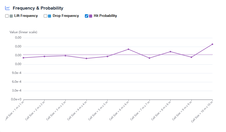
As DORAS utilizes a cellular grid structure instead of a circular ring structure for calculations, and given that the data in the DNV example is rounded in some cases, and given that the measurement of target lengths will vary slightly, some variance between the DNV calculated results and the DORAS calculated results will occur. However, this variance is very small and within a reasonable margin of error. Specifically in relation to the differences between the cellular grid structure and the circular ring structure, an eight square meter grid structure will produce results closest to the results for a ten meter circular ring structure as used in the DNV example. Smaller cellular grid structures will generally produce lower hit consequence results due to the reduction in averaging within the calculation results which are performed over large areas.
The validation process confirms that the DORAS application correctly implements all key calculation methodologies from DNV-RP-F107:
| Calculation Component | DNV - Circular Rings - 10m² | DORAS - Cellular Grid - 8m² | DORAS - Cellular Grid - 10m² |
|---|---|---|---|
| Drop Frequency | 4.81E-02 drops per annum | 4.81E-02 drops per annum | 4.81E-02 drops per annum |
| Lateral Deviation (m) | 1σ = (26.8, 15.8, 8.8, 17.6, 8.8, 5.2) | 1σ = (26.79, 15.84, 8.75, 17.63, 8.75, 5.24) | 1σ = (26.79, 15.84, 8.75, 17.63, 8.75, 5.24) |
| Conditional Target Hit Probability | 1.64E-03 hits per annum | 1.63E-03 hits per annum | 1.42E-03 hits per annum |
| Target Hit Frequency | 1.37E-05 per annum | 1.36E-05 per annum | 1.56E-05 per annum |
| Accumulated Hit Frequency for Energy Levels | >0kJ = 1.37E-05>50kJ = 9.58E-06>100kJ = 7.10E-06>200kJ = 5.18E-06>400kJ = 3.54E-06>800kJ = 2.04E-06 | >0kJ = 1.36E-05>50kJ = 9.49E-06>100kJ = 7.03E-06>200kJ = 5.12E-06>400kJ = 3.51E-06>800kJ = 2.02E-06 | >0kJ = 1.56E-05>50kJ = 1.09E-05>100kJ = 8.09E-06>200kJ = 5.90E-06>400kJ = 4.03E-06>800kJ = 2.33E-06 |
| Target Damage Frequency | D1 = 4.99E-06D2 = 2.50E-06D3 = 6.21E-06 | D1 = 4.95E-06D2 = 2.52E-06D3 = 6.12E-07 | D1 = 5.70E-06D2 = 2.90E-06D3 = 7.04E-07 |

All validated calculation components produce results that match the DNV-RP-F107 Appendix A worked example within acceptable numerical precision limits. Minor differences may occur due to:
- Rounding differences in intermediate calculation steps
- Grid resolution effects in the matrix-based calculation approach (which provides higher resolution than the ring-based method in the DNV example)
- Computational precision differences between manual calculations and automated computational methods
These differences are expected and do not indicate calculation errors, but rather reflect the enhanced precision and resolution capabilities of the application's matrix-based grid system.
The validation process is an ongoing activity. As new features are added or calculation methods are enhanced, validation against the DNV-RP-F107 worked example is repeated to ensure continued accuracy and compliance with the standard.
Frequently asked questions
Common questions about how the calculations work in practice. For DNV-RP-F107 informational queries (what the standard is, how it differs from spreadsheet tools, what outputs it produces), see the DNV-RP-F107 software page.
How does DORAS calculate landing probability per grid cell?
DORAS divides the analysis area into a regular grid (typically 1m × 1m cells) and uses Monte Carlo simulation to model dropped object trajectories. For each simulated drop, the landing position is recorded against the grid; running thousands of iterations builds a per-cell landing probability distribution. The grid resolution gives 100 times finer spatial detail than the traditional 10m concentric-ring approximation used by spreadsheet-based DNV-RP-F107 implementations.
What is Monte Carlo simulation in dropped object analysis?
Monte Carlo simulation models dropped object outcomes by randomly sampling input variables (drop height, lateral deviation, current speed, etc.) thousands of times and aggregating the results into probability distributions. Compared with closed-form calculations, it captures the full statistical spread of possible landing locations and lets DORAS report frequency estimates with quantifiable uncertainty even for low-probability events.
How does grid-based analysis differ from concentric ring methods?
Concentric ring methods (used in many spreadsheet-based DNV-RP-F107 tools) average risk across large bands — typically 10m wide — around each drop point. This works for simple cases but loses fidelity when targets are small, drop points overlap, or drop areas are irregular. Grid-based analysis computes landing probability per cell (1m × 1m by default) and intersects against the actual target geometry, capturing fine spatial detail and supporting multi-source aggregation in a single integrated model.
What inputs does DORAS need to run a study?
A DORAS study needs: (1) the analysis area boundary; (2) drop sources — lifts, drop points and the object types being lifted; (3) target geometry — pipelines (linear) or other equipment (polygon) at risk, with their depth and damage capacity; (4) DNV-RP-F107 reference values for drop frequency, energy distributions and target capacity (editable defaults are supplied); and (5) any site-specific environmental data such as water depth and currents. Templates allow reuse across similar studies.
How long does a typical study calculation take?
A typical offshore facility study with one or two drop points and a single pipeline target completes in seconds. Larger campaigns covering many drop points, multiple object types and several targets can take a few minutes; high-frequency lift studies (over 10,000 drops per lift) auto-enable statistical sampling so calculation times remain tractable. The web interface tracks progress in real time and the calculation engine stores results so reruns are inexpensive after a parameter change.
Next steps
Now that you've seen the methodology, here are three useful next steps:
- See the full DORAS feature set — calculation engine, visualisation, reporting, collaboration.
- Read the DNV-RP-F107 software overview — informational FAQ on the standard and how DORAS implements it.
- Talk to us about a project — get a free 30-day evaluation or scope a campaign.
6. References
- DNV-RP-F107: Risk assessment of pipeline protection. Det Norske Veritas.
- DNV Table 4-1: Conditional probabilities for steel pipelines
- DNV Table 4-2: Conditional probabilities for flexible pipelines
- DNV Table 4-3: Conditional probabilities for umbilicals
- DNV Table 5-4: Energy level probability distributions by object class
- DNV Section 5.3: Energy calculations (Equations 13-16)
- DNV Section A.8: Energy threshold calculations (Equation 3)
- DNV Appendix A: Worked example with proportional distribution methodology
Version 1.2 (July 2026): Updated documentation to reflect the current state of the application, including the new Simple Current Effects methodology and the updated calculation engine architecture.
Version 1.1 (July 2026): Added comprehensive documentation for Simple Current Effects methodology (Section 2.2.1), including current-induced dispersion calculations, quadrature addition statistical combination, and multi-sigma recalculation procedures.
Version 1.0 (Initial Release): Initial methodology documentation covering study creation workflow and all calculation methods per DNV-RP-F107 standards.
This document is maintained as part of the DORAS application documentation.